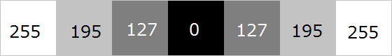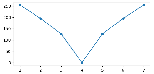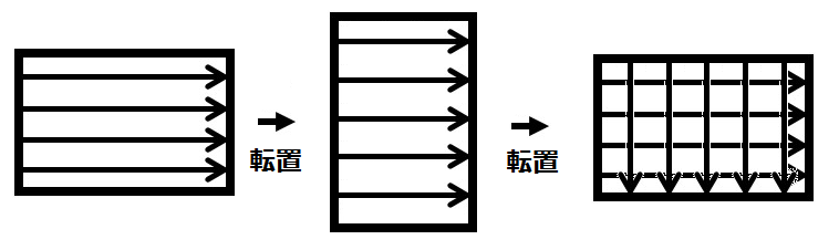
Each result returned by the distributed processing is not made into a PN-sized matrix, but is placed as is. This lightens the processing.
|
1 2 3 4 5 6 7 8 9 10 11 12 13 14 15 16 17 18 19 20 21 22 23 24 25 26 27 28 29 30 31 32 33 34 35 36 37 38 39 40 41 42 43 44 45 46 47 48 49 50 51 52 53 54 55 56 57 58 59 60 61 62 63 64 65 66 67 68 69 70 71 72 73 74 75 76 77 78 79 80 81 82 83 84 85 86 87 88 89 90 91 92 93 94 95 96 97 98 99 100 101 102 103 104 105 106 107 108 109 110 111 112 113 114 115 116 117 118 119 120 121 122 123 124 125 126 127 128 129 130 131 132 133 134 135 136 137 138 139 140 141 142 143 144 145 146 147 148 149 150 151 152 153 154 155 156 157 158 159 160 161 162 163 164 165 166 167 168 169 170 171 172 173 174 175 176 177 178 179 180 181 182 183 184 |
import random import math import time import gc import numpy as np from multiprocessing import Pool np.set_printoptions(threshold=np.inf) random.seed(1) XX = 0 YY = 1 ZZ = 2 core = 6 #total particle num PN = 10000 #--------------------------------------------------- # # parameter : divide_N # # The number of particles per side of a small square # divided for the splitting process when creating a # large PN^2 region with all particles PN. # # The smaller the setting, the more it will be divided # into many smaller jobs. #--------------------------------------------------- divide_N = 1000 xyzV = [[0 for i in range(3)] for j in range(PN)] xyzP = np.zeros((PN,3)) xyzF = np.zeros((PN,3)) def wrapper(args): return calc_XY_start_end(*args) def find_pair(): global core global PN global xyzF global xyzP worklist = [] thread = 0 remainder = PN % divide_N quotient = PN // divide_N if remainder != 0: #ex PN=11, divide_N=4, remainder=3, quotient=2 quotient = quotient + 1 # 2 -> 3 extra = divide_N - remainder # 1 X_st = 0 X_ed = 0 Y_st = 0 Y_ed = 0 Thead_num = 0 sum_f = np.zeros((PN,PN,3)) for Xn in range(0,quotient): for Yn in range(0,Xn+1): worklist.append([Xn, Yn, quotient, remainder, divide_N, extra]) Thead_num = Thead_num + 1 #---------------------------------------- #local_force = calc_XY_start_end(Xn, Yn, quotient, remainder, divide_N, extra) #---------------------------------------- #start thread. results is callback in array. p = Pool(core) callback = p.map(wrapper, worklist) p.close() t1 = 0 for Th in range(0,Thead_num): xn_l = callback[Th][0] yn_l = callback[Th][1] xxst = callback[Th][2] xxed = callback[Th][3] yyst = callback[Th][4] yyed = callback[Th][5] local_force = callback[Th][6] time_sta = time.time() sb = local_force.shape ten = -1 * local_force.transpose(1,0,2) tensb = ten.shape sum_f[yyst:yyst+sb[0], xxst:xxst+sb[1]] += local_force if xn_l != yn_l: sum_f[xxst:xxst+tensb[0], yyst:yyst+tensb[1]] += ten time_end = time.time() t1 =t1 + (time_end - time_sta) print ("=====t1=",t1) print(np.sum(sum_f)) #mmm = sum_f.sum(axis=1) #xyzF = xyzF + mmm def calc_XY_start_end(Xn, Yn, quotient, remainder, divide_N, extra): global PN global xyzP if Xn != quotient-1 and remainder != 0 or remainder == 0: X_st = Xn*divide_N X_ed = (Xn+1)*divide_N-1 else: X_st = Xn*divide_N - (divide_N - remainder) X_ed = (Xn+1)*divide_N - (divide_N - remainder) -1 if Yn != quotient-1 and remainder != 0 or remainder == 0: Y_st = Yn*divide_N Y_ed = (Yn+1)*divide_N-1 else: Y_st = Yn*divide_N - (divide_N - remainder) Y_ed = (Yn+1)*divide_N -(divide_N - remainder) -1 Xa = np.arange(X_st,X_ed+1) Ya = np.arange(Y_st,Y_ed+1) mx1,my1 = np.meshgrid(Xa,Ya) local_xyz = xyzP[mx1]-xyzP[my1] distance_a = np.linalg.norm(local_xyz, axis=2) tmp_d = distance_a[:,:,np.newaxis] tmp_f = local_xyz/tmp_d tmp_f = np.nan_to_num(tmp_f,0) #extra clear if remainder != 0: if Xn + 1 == quotient: for dd in range(0,extra): tmp_f[:,dd] = 0 if Yn + 1 == quotient: for dd in range(0,extra): tmp_f[[dd]] = 0 return Xn,Yn,X_st,X_ed,Y_st,Y_ed,tmp_f def init_lattice(): global xyzF global xyzP pnum = 0 while pnum < PN: xyzP[pnum][XX] = random.uniform(-1,1) xyzP[pnum][YY] = random.uniform(-1,1) xyzP[pnum][ZZ] = random.uniform(-1,1) xyzF[pnum][XX] = random.uniform(-1,1) xyzF[pnum][YY] = random.uniform(-1,1) xyzF[pnum][ZZ] = random.uniform(-1,1) pnum += 1 def results_sum(): global xyzF pnum = 0 total_F = 0 # while pnum < PN: # total_F = total_F + xyzF[pnum][XX] # total_F = total_F + xyzF[pnum][YY] # total_F = total_F + xyzF[pnum][ZZ] # pnum += 1 # # print (total_F) if __name__ == "__main__": init_lattice() find_pair() results_sum() |